Connect this book to a runtime
If you would like to change something or repeat the code execution, BinderHub can help you with that! Hover the [🚀] button above and request an execution runtime to re-execute this book while you are reading it.
🔪 NumPy basics
Visit the reference blog post for more examples.
If you have
lolvizand its dependencies intalled properly,arrayvizfunction will show you a visual representation of the array. If not, you will see the
import numpy as np
# Import NumPy
import numpy as np
# A tiny exception block
try:
from lolviz import listviz as lolist
except:
print('Lolviz is not enabled.')
# Pictorial representation of arrays
def arrayviz(inp):
try:
out = lolist(inp)
return out
except Exception as e:
print(inp)
# Let's create an array
my_array = np.array([11,22,33,44,55,66,77,88])
# Other data types
# my_array = np.array([11,22,33,44,55,66,77,88],dtype=np.complex64)
# my_array = np.array([11,22,33,44,55,66,77,88],dtype=np.float64)
# Transpose of a 1D aray has the same shape
# my_array = my_array.T
print("Number of dimensions: ", my_array.ndim)
print("Array shape (row,col): ", my_array.shape)
print("Array size (number of elements): ", my_array.size)
print("Array data type", my_array.dtype)
print("Item size in bytes", my_array.itemsize)
arrayviz(my_array)
Number of dimensions: 1
Array shape (row,col): (8,)
Array size (number of elements): 8
Array data type int64
Item size in bytes 8

'''
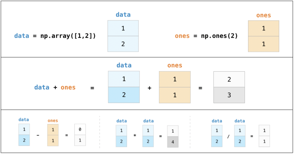
Array arithmetic operations
'''
my_array = np.array([11,22,33,44,55,66,77,88])
your_array = np.array([1,2,3,4,5,6,7,8]) # Must be the same length with my_array
print('Add: ', my_array + your_array,
'\nSubtract: ', my_array - your_array,
'\nMultiply: ', my_array * your_array,
'\nDivide: ', my_array/your_array,
'\nFloor divide: ', my_array//your_array,
'\nPower: ', my_array**your_array
)
Add: [12 24 36 48 60 72 84 96]
Subtract: [10 20 30 40 50 60 70 80]
Multiply: [ 11 44 99 176 275 396 539 704]
Divide: [11. 11. 11. 11. 11. 11. 11. 11.]
Floor divide: [11 11 11 11 11 11 11 11]
Power: [ 11 484 35937 3748096
503284375 82653950016 16048523266853 3596345248055296]
Array creation routines
array empty zeros ones linspace arange full
my_array = np.arange(11,88,11)
'''
Start from 11 and return values with increments
of 11 until 89 is reached.
'''
print('np.arange: ')
arrayviz(my_array)
np.arange:

my_array = np.linspace(11,88,5).astype('int16') # Without .astype, it'll return float
'''
Return 8 evenly spaced numbers over 11-88 interval
'''
print('np.linspace: ')
arrayviz(my_array)
np.linspace:

zrs = np.zeros(8) # Returns of array of zeros with 8 elements
print('np.zeros: ')
arrayviz(zrs)
np.zeros:

ones = np.ones(8).astype('int16') # Returns of array of ones with 8 elements
print('np.ones: ')
arrayviz(ones)
np.ones:

full = np.full(8,10) # Returns of array of desired value with 8 elements
print('np.full: ')
arrayviz(full)
np.full:

empty = np.empty(8)
'''
Returns of array of 8 elements w ithout EXPLICITLY INITIALIZING it with certain values
The values we'll see are arbitrary, i.e. as they exist in the memory address allocated for our array.
'''
print('np.empty: ')
arrayviz(empty)
np.empty:

NumPy provides us with:
A versatile chef’s knife to slice our data as we like (slicing)
All the cookware to organize them (data types)
Easy way to access what we need, when we need (indexing)
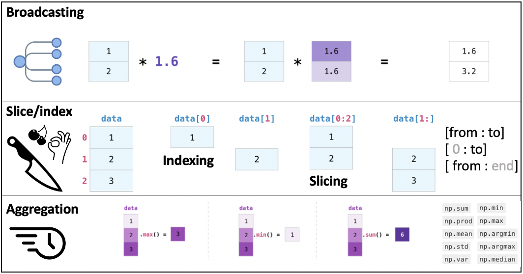
Broadcasting
'''
Broadcasting
'''
my_array = np.arange(11,89,11)
my_array2 = my_array # WARNING! This will create a "shallow" copy (just another pointer to the same array)
my_array2 *= 2 # Equivalent of my_array = my_array * 2
arrayviz(my_array2)

Copying
'''
As you can see, changes we made on my_array2 reflected on my_array as well.
'''
arrayviz(my_array)

'''
To create an "independent" clone, we can use deep copy
'''
import copy
my_array = np.arange(11,89,11) # Create a fresh instance
my_array2 = copy.deepcopy(my_array) # Now my_array2 is NOT a pointer to my_array
my_array2 *= 2 # // is floor devision operator
print('Original: ', my_array, 'Deep-copied, modified: ',my_array2)
Original: [11 22 33 44 55 66 77 88] Deep-copied, modified: [ 22 44 66 88 110 132 154 176]
Indexing
'''
Cherrypick an element
'''
first = my_array[0]
last = my_array[-1]
print('First element: ', first, 'Last element', last)
First element: 11 Last element 88
Slicing
'''
Slice
'''
portion_from_start = my_array[:3] # Eqv my_array[0:3]
print('First portion: ', portion_from_start)
portion_from_end = my_array[5:] # Eqv my_array[5:-1]
print('Last portion: ', portion_from_end)
interleave_odd = my_array[::2] # Eqv my_array[0::2]
print('Interleaved odd: ', interleave_odd)
interleave_even = my_array[1::2]
print('Interleaved even: ', interleave_even)
reverse = my_array[::-1]
print('Reversed: ', reverse)
First portion: [11 22 33]
Last portion: [66 77 88]
Interleaved odd: [11 33 55 77]
Interleaved even: [22 44 66 88]
Reversed: [88 77 66 55 44 33 22 11]
In-place filtering
'''
In-place filtering
'''
my_array = np.arange(11,89,11)
my_array[((my_array<50) & (my_array>20))] = 0
arrayviz(my_array)

Aggregation functions
'''
Aggregation functions
'''
my_array = np.arange(11,89,11)
print(
"\n min: ", my_array.min(), # Returns the minimum element itself
"\n max: ", my_array.max(), # Returns the maximum element itself
"\n argmin: ", my_array.argmin(), # Returns the index of the minimum element in the array
"\n argmax: ", my_array.argmax(), # Returns the index of the maximum element in the array
"\n std: ", my_array.std(), # Returns the standard deviation of the array
"\n sum: ", my_array.sum(), # Returns the sum of the elements in the array
"\n prod: ", my_array.prod(), # Returns the product of the elements in the array
"\n mean: ", my_array.mean()
)
arrayviz(my_array)
min: 11
max: 88
argmin: 0
argmax: 7
std: 25.20416632225712
sum: 396
prod: 8642950081920
mean: 49.5

NumPy aggregation vs Python native
To see whether np.max() is faster, first we need to create a larger array. Then, we’ll use %timeit magic to see which one outperforms the other 🏎
test = np.random.rand(10000)
'''
One important note about random number generation
If you'd like that "randomness" reproduce, you need to
seed numpy random number generator
'''
np.random.seed(123)
print('Numpy aggregation')
%timeit -n 500 mx = test.max()
print('Python native')
%timeit -n 500 mx2 = max(test)
Numpy aggregation
5.53 µs ± 368 ns per loop (mean ± std. dev. of 7 runs, 500 loops each)
Python native
713 µs ± 9.49 µs per loop (mean ± std. dev. of 7 runs, 500 loops each)
🔊 Acoustic dissonance

1️⃣ Shopping
Know your data at least at the level you are dealing with it!
Please bear with me here for a while, because we’ll be dealing with *wav files at a somewhat low-level.
For demonstration, we will write a small function that can read and parse *.wav files into a NumPy array.
This step has no coding. Yet, having some insights about your data beforehand gives you a great headstart for the next step!
So, in a manner of speaking, semantics will do 🙃 If Nouvelle Vague is not your cup of tea, maybe this is:
When you try your best, but you can't debug
When
p<0.0000000000000000000000000001, and you are not comfortable with it
When you read the code, but it seems OK
Stuck in limbo
When you smell something fishy about your custom reader
When you analyze for days, but it goes to waste
What could be worse?
Data standards will guide you home
And validate your data
And you won't need to fix it
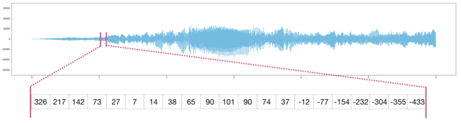
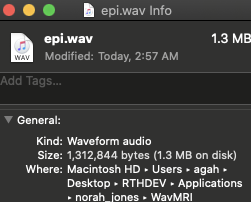
👉 WavMRI/EPI.wav is a stereo (2 channels) recording of the acoustic noise EPI gradient pulses make, sampled at 44.1kHz for 7.42 seconds. Saved at 16bit depth. This is how I know (Garageband):
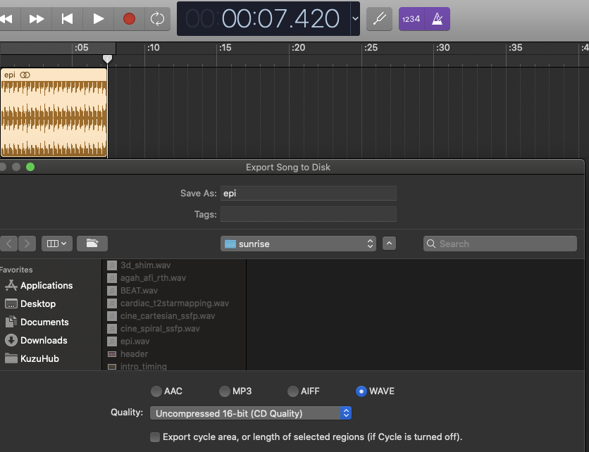
Thus, we should expect an array with a length of 655094 = 327547 (samples) X 2 (stereo means 2 channels)
The number of bytes per sample is 16(bits)/8 = 2
The *.wav file contains these information pieces in the header, describing the format of the sound information stored in the data chunk:
field name |
description |
|---|---|
|
The number of channels in the wave file (mono = 1, stereo = 2) |
|
The number of bytes per sample |
|
The number of frames per second (a.k.a sampling frequency) |
|
The number of frames in the data stream (a.k.a number of samples) |
|
A string object containing the bytes of the data stream |
2️⃣ Mise en place
We did the shopping!
*.wav is still a popular data format among music producers. So we are using fresh ingridients to compose our magnetic melodies, way to go! 👩🍳
Now it is time to combine our *.wav knowledge with our NumPy skills to create an object that we can hear.
Before coding, we should relate our knowledge about the data with the docs of the module we’ll use to read it!
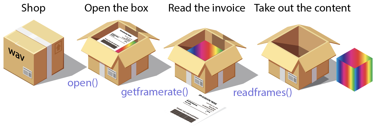
👉 Click this line to expand the API documentation of wave module. See how objects returned by open can access header and data of a *.wav file!

from wave import open as open_wave
'''
OPEN THE BOX
Open "WavMRI/EPI.wav" file in read mode
'''
fp = open_wave("../WavMRI/EPI.wav", "r")
'''
READ THE INVOICE
Use wave module's methods to read metadata
'''
nchannels = fp.getnchannels()
nframes = fp.getnframes()
framerate = fp.getframerate()
sampwidthbyte = fp.getsampwidth()
print("nChannels: ", nchannels , "\nnFrames: " , nframes, "\nframerate: ",framerate, "\nsampwidth in bytes: ",sampwidthbyte)
'''
TAKE OUT THE CONTENTS
We read machine-byte ordered data into
AN ARRAY OF BYTES (STRING ENCODED)
'''
z_str = fp.readframes(nframes)
'''
CLOSE THE BOX
'''
fp.close()
'''
SEE WHAT IT LOOKS LIKE
Expected number of frames per channel was 327547 (fSamp * duration)
Expected content size was about 1.3MB
'''
print( "BOX CONTENT SIZE", len(z_str), '\nBOX CONTENT: ', z_str[:20])
nChannels: 2
nFrames: 327547
framerate: 44100
sampwidth in bytes: 2
BOX CONTENT SIZE 1310188
BOX CONTENT: b':#:#e;e;\x0eQ\x0eQZbZb\xc0n\xc0n'
'''
MAKE THE CONTENT USEFUL BASED ON WHAT WE LEARNT FROM THE INVOICE!
We already know that the data is recorded in 16bit. But we can also
infer it from the metadata
'''
print('Each entry is ', sampwidthbyte * 8, ' bits. (1 byte = 8 bits)')
'''
CONVERT DATA INTO USEFUL INFORMATION
We can't use np.array, we need to use
frombuffer as we are reading machine-byte
ordered data.
'''
sgnl = np.frombuffer(z_str, dtype=np.int16)
'''
PLOTLY EXPRESS
One line of code for interactive plots!
NOTE that I plot 1 in every 50 samples. This is just to make things faster.
'''
import plotly.express as px
fig = px.line(sgnl[::50],template='plotly_dark',title='STEREO')
fig
Each entry is 16 bits. (1 byte = 8 bits)
'''
TAKE OUT ONLY ONE CHANNEL
Order: Ch1, Ch2, Ch1, Ch2....
SLICE
'''
sgnl = sgnl[::2]
# Again, plotting 1/50 samples
fig = px.line(sgnl[::50],template='plotly_dark',title='MONO')
fig
'''
MAKE AUDIO
Use IPython's Audio module
'''
from IPython.display import Audio
hear = Audio(data=sgnl,rate=framerate)
hear
🎶 Helper functions
read_wave(filename)Reads *.wav file to return:ysAudio signal (mono)framerateSampling frequencytsTime points
normalize(ys,amp)Normalizes audio signal amplitude to a user defined range (amp):ysNormalized audio signal
make_audio(ys,amp)Takesysandframerateand returns an eenie meenie media player.
load_audio(filename,rate_factor=1,duration=0,volume=1)Inputs
filename Wav file
rate_factor Multiplied with sampling freq during
make_audio step. (>1 higher & faster, vice versa)duration Trims audio [0:duration], yeah just that.
volume Normalization range (Use 1 max)
Output (dict)
['signal']Audio signal['time']Time pts['fsamp']Sampling frequency['duration']Shows you the importance of reading docs. Duration of the audio in seconds['play']Weeny IPython media player that can play the loaded file
fastforward(ys, factor)Speeds up the audio by re-arranging sound samples.
def read_wave(filename):
'''
Now we have a tiny function that can
load 16bit wav files into a numpy array.
It also returns its time axis and sampling
frequency.
'''
fp = open_wave(filename, "r")
nchannels = fp.getnchannels()
nframes = fp.getnframes()
framerate = fp.getframerate()
z_str = fp.readframes(nframes)
fp.close()
# We assume that data is always 16bits. Change this to
# int64 and see what happens :)
ys = np.frombuffer(z_str, dtype=np.int16)
if nchannels == 2:
ys = ys[::2]
ts = np.arange(ys.size)/framerate
return ys, framerate,ts
def normalize(ys, amp=1.0):
'''
Amplitude range of the *.wav files we load
is random. This function will be useful when
we are combining tracks and would like to hear
some of them less/more in the mix.
'''
# TASK: Use NumPy aggregation functions :)
high, low = abs(max(ys)), abs(min(ys))
# Broadcasting
return amp * ys / max(high, low)
def make_audio(ys,frame_rate):
'''
To hear *.wav files we load into np.arrays,
we need to create an IPython Audio object.
'''
audio = Audio(data=ys,rate=frame_rate)
return audio
def load_audio(filename,rate_factor=1,duration=0,volume=1):
'''
filename: *.wav file
rate_factor: Changes sampling frequency at the audio
generation step. This changes the frequency
but also impacts the play duration.[0,inf)
duration: Trims audio at a desired time point (s).
volume: Normalizes signal amplitude [0-1]
'''
ys, fs, ts = read_wave(filename)
if duration is not 0:
# Type casting, broadcasting
cut = np.floor(fs*duration).astype('int')
# Slicing
ys = ys[:cut]
ts = ts[:cut]
ys = normalize(ys,volume)
audio = dict(
signal = ys,
time = ts,
fsamp = fs,
duration = ys.size/fs,
play = make_audio(ys,fs*rate_factor))
return audio
def fastforward(ys, factor):
'''
Fast forwards the audio (ys) without messing with the
sampling frequency.
'''
idx = np.round( np.arange(0, ys.size, factor) )
idx = idx[idx < ys.size].astype(int)
return ys[ idx.astype(int) ]
The following code block requires a runtime, therefore won’t be rendered offline. You can toggle it to see the code. Please start an interactive session if you would like to execute.
'''
A really simple interactive visualization
If you'd like to learn more about interactive dataviz
https://github.com/agahkarakuzu/datavis_edu
'''
import plotly.graph_objects as go
from pandas import DataFrame as pd
from ipywidgets import interact
'''
USE load_audio
'''
temp = load_audio('../WavMRI/EPI.wav')
df = pd.from_dict(dict(time = temp['time'][::50], signal = temp['signal'][::50]))
fig = px.line(df,x='time',y='signal',
template='plotly_dark', title="EPI acoustic noise, Normalized")
fig.update_traces(line=dict(color='limegreen'),opacity=0.7)
fig.update_yaxes(range=[-1,1])
# All Plotly charts have click, hover and zoom events which can be accessed
# by go.FigureWidget using Jupyter Widgets
# Here we create a FigureWidget object (f2) that communicates with our interactive
# figure (fig).
f2 = go.FigureWidget(fig)
# @interact decorates the volume_plot function. y=(0.0,1.0) informs ipywidgets to
# create a slider, whose value (y) will update f2.data[0].y (y data of the plotly figure object)
# whenever the slider is changed.
@interact(y=(0.0,1.0))
def volume_plot(y):
'''
CALL normalize each time the slider is moved
'''
# f2.data[0] means that the first trace that is stored in this figure.
# .y denotes the y axis, to update x, f2.data[0].x etc.
# There are many other attributes we can update, including the figure layout
# axes limits, portion of the data displayed...
# For more examples: https://plotly.com/python/figurewidget/
f2.data[0].y = normalize(temp['signal'][::50],y)
Music & frequency
Do you remember Nokia 3310 music composer? See this masterpiece!
If you don’t know what Nokia 3310 is, it means that I’m getting old. Anyway, I just wanted to appreciate the “sophistication” in that nostalgic composer. You’ll see that adjusting tone, duration & tempo is not that easy.
🧲 Jingle gradients
def jingle_gradients(filename, dur):
samp_s = load_audio(filename,rate_factor=1,duration=dur, volume=1)
# Feel free to change this notes array :)
fake_notes = np.array([1,1,1,1,1,1,1.06**3,
0.94**4,0.94**2,1,1.06,
1.06,1.06,1,1,1,0.94**2,
0.94**2,0.94**2,1,0.94**2,
1.06**3])
'''
I called them fake because we are changing them by speeding up
the audio signal. This does not easily allow us to set durations
(notes change otherwise).
1.06 is the factor for one halftone up (sharp)
1.06**2 --> 2 halftones up
0.94 is the factor for one halftone down (flat)
0.94**3 --> 3 halftones down etc.
'''
a = fastforward(samp_s['signal'], 1)
for note in fake_notes:
b = fastforward(samp_s['signal'], note)
a = np.hstack((a,b))
return a
'''
Change the MRI sample to play Jingle Bells
with a different sequence :)
'''
#jingle = jingle_gradients('../WavMRI/CINE_cartesian_SSFP.wav',0.2)
jingle = jingle_gradients('../WavMRI/EPI.wav',0.2)
#jingle = jingle_gradients('../WavMRI/BEAT.wav',0.2)
'''
If you add up different sequence noise, it won't be harmonic.
'''
make_audio(jingle,44100)
'''
Amplitude modulation
'''
def f(t, f_c, f_m, beta):
'''
t = time
f_c = carrier frequency
f_m = modulation frequency
beta = modulation index
'''
return np.sin(2*np.pi*f_c*t - beta*np.cos(2*f_m*np.pi*t))
def to_integer(signal):
'''
Take samples in [-1, 1] and scale to 16-bit integers,
values between -2^15 and 2^15 - 1.
'''
return np.int16(signal*(2**15 - 1))
N = 44100
x = np.arange(3*N) # three seconds of audio
siren = f(x/N, 1500, 3, 100)
make_audio(siren,44100)
🙌 Exercise: Wav signal & pure tones
Generate a pure tone using np.sin that has the same duration with a sound sample of your choice, then multiply/add them to see what it gives. You need to unlock the code cell first by achieveing this simple task:
tduration=
'''
TASK: Assign tduration with the duration of the signal (in seconds, but be accurate!)
'''
👂 Test your musical ear
Change the sin_freq with small increments, and see after how many Hz you’ll distinguish the sine tone from the SPGR noise. 164Hz is the next note (E3). If you can tell them before that, you have an ear for eastern music, if you cannot tell it after 164Hz, you may be tone deaf 👀
Set
sin_freqto 155 (D#3)Load
3DSPGR_TR12ms.wavUse
result = my_sound['signal'] + sin_wavePlay and see if they are attuned ;)
Hint
You can use this approach to find out the dominant sound frequency of a pulse sequence of your choice.
Exercise
Use click to show toggle below to see the exercise.
# TASK: Assign tduration with the duration of the signal (in seconds, but be accurate!)
#my_sound = load_audio('../WavMRI/3DSPGR_TR12ms.wav') # Select one from WavMRI folder
#tduration=
#sin_freq = 10
#Choose a lower (e.g. 2) or a higher (e.g. 1000) sin_freq and see how they affect the output.
#sf = my_sound['fsamp']
#sin_wave = (np.sin(2*np.pi*np.arange(sf*tduration)*sin_freq/sf))/2
# Tip: You can try other trigonometric functions in numpy as well :)
#result = my_sound['signal'] * sin_wave
# Tip: Add, subtract & multiply your sound with this sin_wave
#make_audio(result,my_sound['fsamp']) # Hear it!
🙌 Exercise: Convolution
Ever heard about reverbation? It is a highly popular sound effect for instruments and vocals.
Reverb lets you transport a listener to a concert hall, a cave, a cathedral, or an intimate performance space.
Sounds exactly like what we need in 2021. We have some time domain impulse responses (IR) that can even take you to outer space (WavIR/OnAStar.wav) 🌟 Wait… What’s a time-domain IR? Gunshot, clap, balloon pop… You can imagine how these sounds “characterize” their environment. Gunshot in a studio vs gunshot in a large hallway. When you convolve your audio with the former one, you’ll get a “dry” sound. Convolution with the latter one yields a “wet” sound.
See the contents of WavIR folder, select one of them, then convolve it with a sound from WavMRI, WavGuitar or WavVocal
You will use np.convolve:
Signature: np.convolve(a, v, mode='full')
Docstring:
Returns the discrete, linear convolution of two one-dimensional sequences.
The convolution operator is often seen in signal processing, where it
models the effect of a linear time-invariant system on a signal [1]_. In
probability theory, the sum of two independent random variables is
distributed according to the convolution of their individual
distributions.
If `v` is longer than `a`, the arrays are swapped before computation.
Exercise
Use click to show toggle before to see the exercise.
#Perform convolution here, then play it!
a = load_audio('../WavVocal/SUNRISE_BENGU.wav')
# v = load_audio('WavIR/your_choice_of_IR.wav')
# convolved = use np.convolve here
# make_audio(convolved,44100)
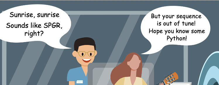
Let's hear NOt RApid Honestly JOyful NEvertheleSs (NORAH JONES) sequence
But first, we will combine the guitar melody (🎸 WavGuitar/SUNRISE.wav) with vocals 🎙 artfully recorded by Bengu Aktas exclusively for this course. Thank you Bengu!
vocal = load_audio('../WavVocal/SUNRISE_BENGU.wav')
vocal['play']
guitar = load_audio('../WavGuitar/SUNRISE_GUITAR.wav')
guitar['play']
'''
Remember array arithmetics, arrays should be of equal size
We can use np.padding on vocal
'''
pad_size = guitar['signal'].size - vocal['signal'].size # Find out how much longer is the guitar track
vocal_padded = np.pad(vocal['signal'], (0, pad_size), 'constant') # Add that many zeros at the end of the vocal track
make_audio(vocal_padded + guitar['signal'],44100) # Make a new audio by adding them
👩🎤 NORAH JONES
Time to hear the acoustic noise NORAH JONES sequence makes and hear (imaginary) feedback from Norah Jones
Pulse sequence
from IPython.display import IFrame
vid = IFrame('https://www.youtube.com/embed/EOBiyV55MNg',560,315)
vid
We have two problems to solve
Duration The original duration of the first verse (Sunrise, sunrise, looks like morning in your eyes…) is about 13 seconds (
WavGuitar/SUNRISE.wav), but NORAH JONES sequence played it for 4 seconds only. Not that slow afterall :)Frequency 4 different tones we heard were supposed to match the keynotes of the original chords, but not all of them did.
target = load_audio('../REMIX/SUNRISE_SPGR_VERSE1.wav')
target['play']
3️⃣ Bring in the chefs
To go from the time to the frequency domain, we’ll invite SciPy chefs to help us out with signal processing.
from scipy import signal
from scipy.fft import fftshift, fft, ifftshift, ifft
import scipy.fftpack as fftpack
import plotly.graph_objects as go
Frequency spectrum
'''
FREQUENCY SPECTRUM
fftshift(fft(mri_orig['signal'])) --> 1D FFT
fftshift(fftpack.fftfreq(mri_orig['signal'].size)) --> Sample frequencies
'''
mri_orig = load_audio('../WavMRI/EPI.wav')
'''
Try other sequences!
BEAT.wav
AFI.wav
LOC_siemens.wav
LOC_SSFP.wav
RT_Shim.wav
...
'''
from pandas import DataFrame as pd
# 1D FFT
X = fftshift(fft(mri_orig['signal']))
# Sample frequencies
freqs = fftshift(fftpack.fftfreq(mri_orig['signal'].size)) * mri_orig['fsamp']
df = pd.from_dict(dict(
Frequency = freqs,
Magnitude = X.real,
Phase = np.angle(X)/np.pi
))
# Real component (yellow)
# You can change y='Phase to show phase instead'
fig = px.line(df,x='Frequency',y='Magnitude',
template='plotly_dark', title="Frequency Spectrum (0-20kHz as fs is 44.1kHz), please zoom in.")
fig.update_traces(line=dict(color='yellow'),opacity=1)
fig